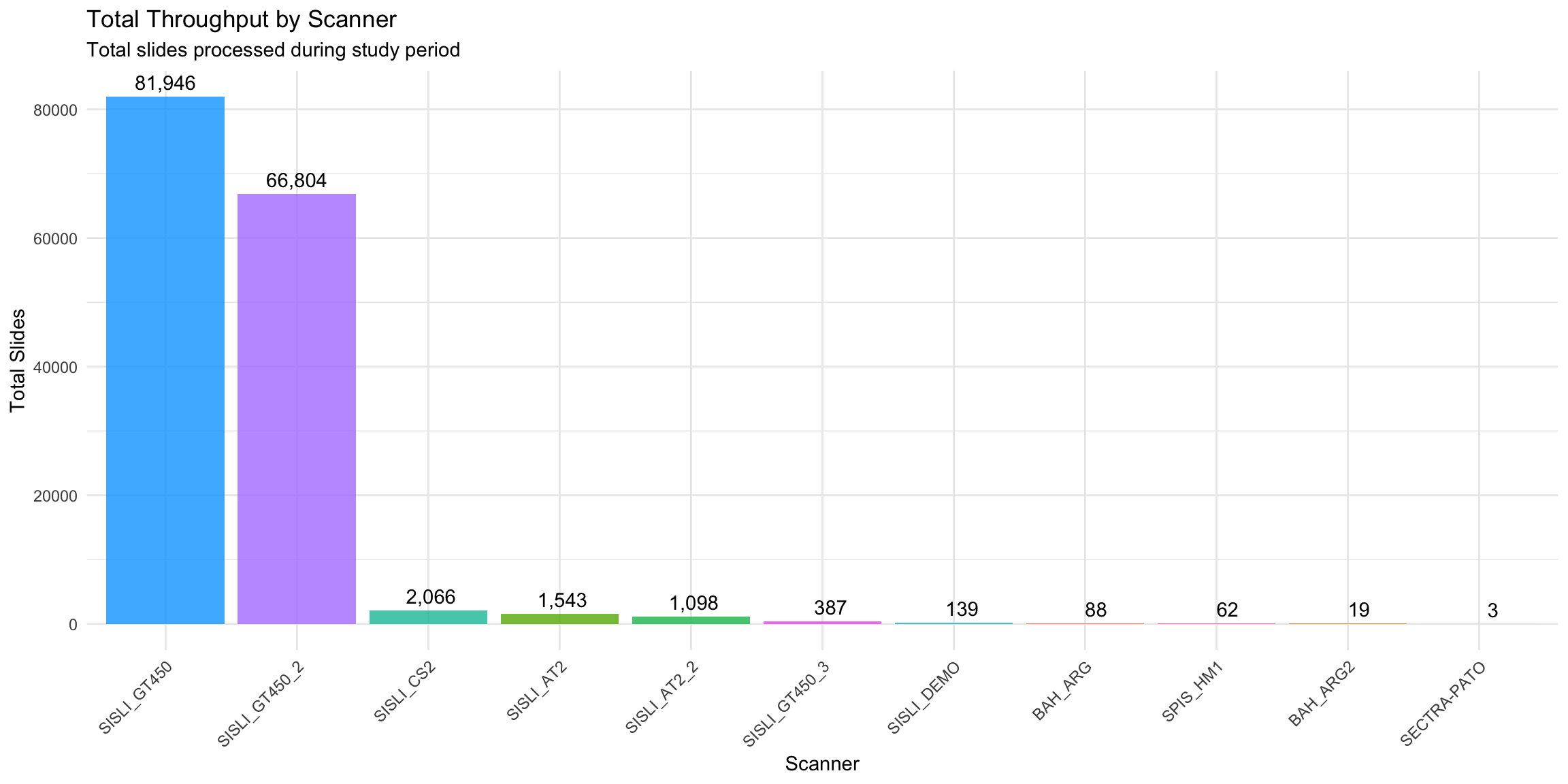
| Scanner | Total Slides | Avg Daily Slides | Time/Slide (hrs) | Utilization (%) | Efficiency Score |
|---|---|---|---|---|---|
| SISLI_GT450 | 81946 | 5.0 | 0.009 | Inf | 8885711 |
| SISLI_GT450_2 | 66804 | 9.0 | 0.011 | Inf | 6004854 |
| SISLI_CS2 | 2066 | NA | NA | NA | NA |
| SISLI_AT2 | 1543 | NA | NA | NA | NA |
| SISLI_AT2_2 | 1098 | NA | NA | NA | NA |
| SISLI_GT450_3 | 387 | 22.5 | 0.005 | 200 | 36519 |
| SISLI_DEMO | 139 | NA | NA | NA | NA |
| BAH_ARG | 88 | NA | NA | NA | NA |
| SPIS_HM1 | 62 | NA | NA | NA | NA |
| BAH_ARG2 | 19 | NA | NA | NA | NA |
| SECTRA-PATO | 3 | NA | NA | NA | NA |
16 Scanner Performance Deep-Dive
16.1 Introduction
This page analyzes the performance of our scanners: GT450 (x2) and AT2 (x2).
Benchmarks (Leica GT450): - Theoretical Speed: < 32 seconds per slide (15mm x 15mm @ 40x). - Target Throughput: 81 slides/hour. - Real-World Reality: Throughput often 30-40 slides/hour due to loading, focus, and network transfer. - Staffing: Industry standard is 1 FTE per 3-4 high-throughput scanners.
We evaluate: 1. Throughput: Slides scanned per hour. 2. Utilization: Active scanning time vs. idle time. 3. Reliability: Frequency of errors or rescans (Target Error Rate: < 1.5%). - Load Balancing: Optimize slide distribution across scanners - ROI Analysis: Calculate cost-effectiveness of each scanner - Capacity Planning: Determine when additional scanners are needed
16.2 Load Data and Run Analysis
16.2.1 IT Infrastructure Impact
The “pipeline” speed is often limited by network bandwidth: - 1 GbE Network: ~15 seconds transfer per slide. - 10 GbE Network: ~1.5 seconds transfer per slide.
Pathologist Note: Fast scanners on a slow network will still result in delayed images. The “bottle” (scanner) might be wide, but the “neck” (network) can be narrow.
16.3 Single Scanner Performance
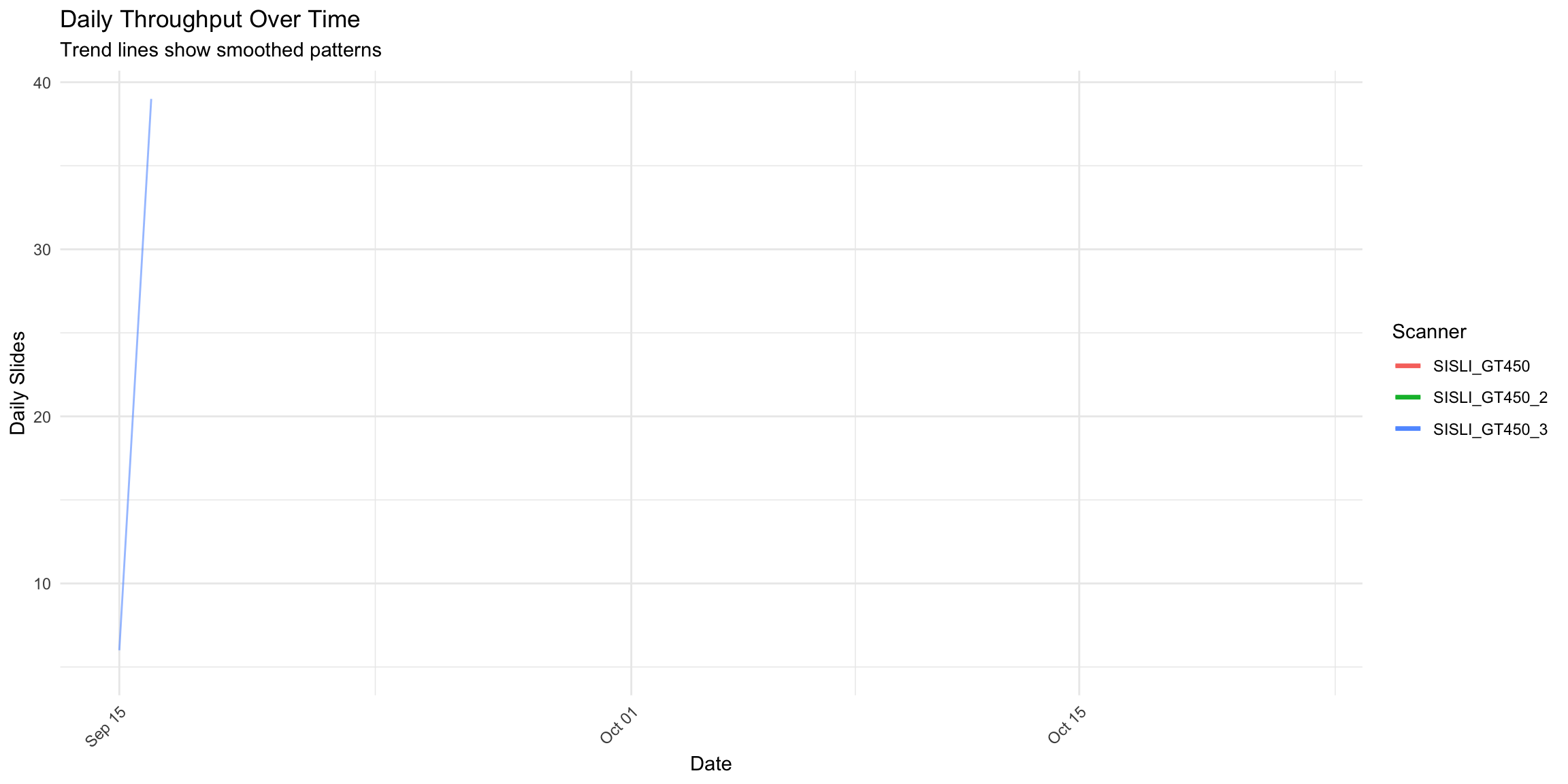
This plot shows the number of slides processed by each scanner per day.
Pathologist Note: Look for consistency. A “sawtooth” pattern (high peaks, deep valleys) often indicates batching behavior or reliability issues, whereas a flat line indicates smooth, optimized production.
16.4 Scanner Performance Metrics
16.5 Total Throughput
16.6 Scanner Efficiency
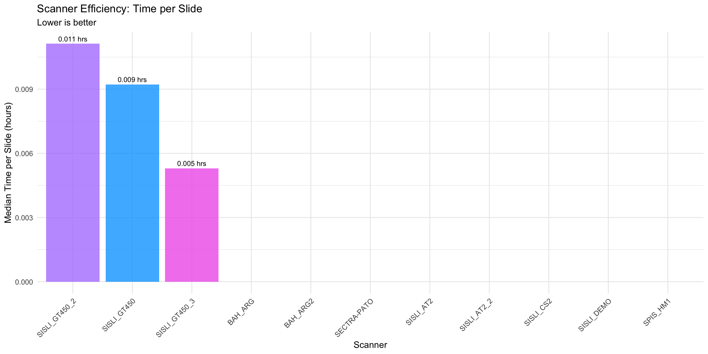
Lower time per slide indicates better efficiency.
16.7 Utilization Rate
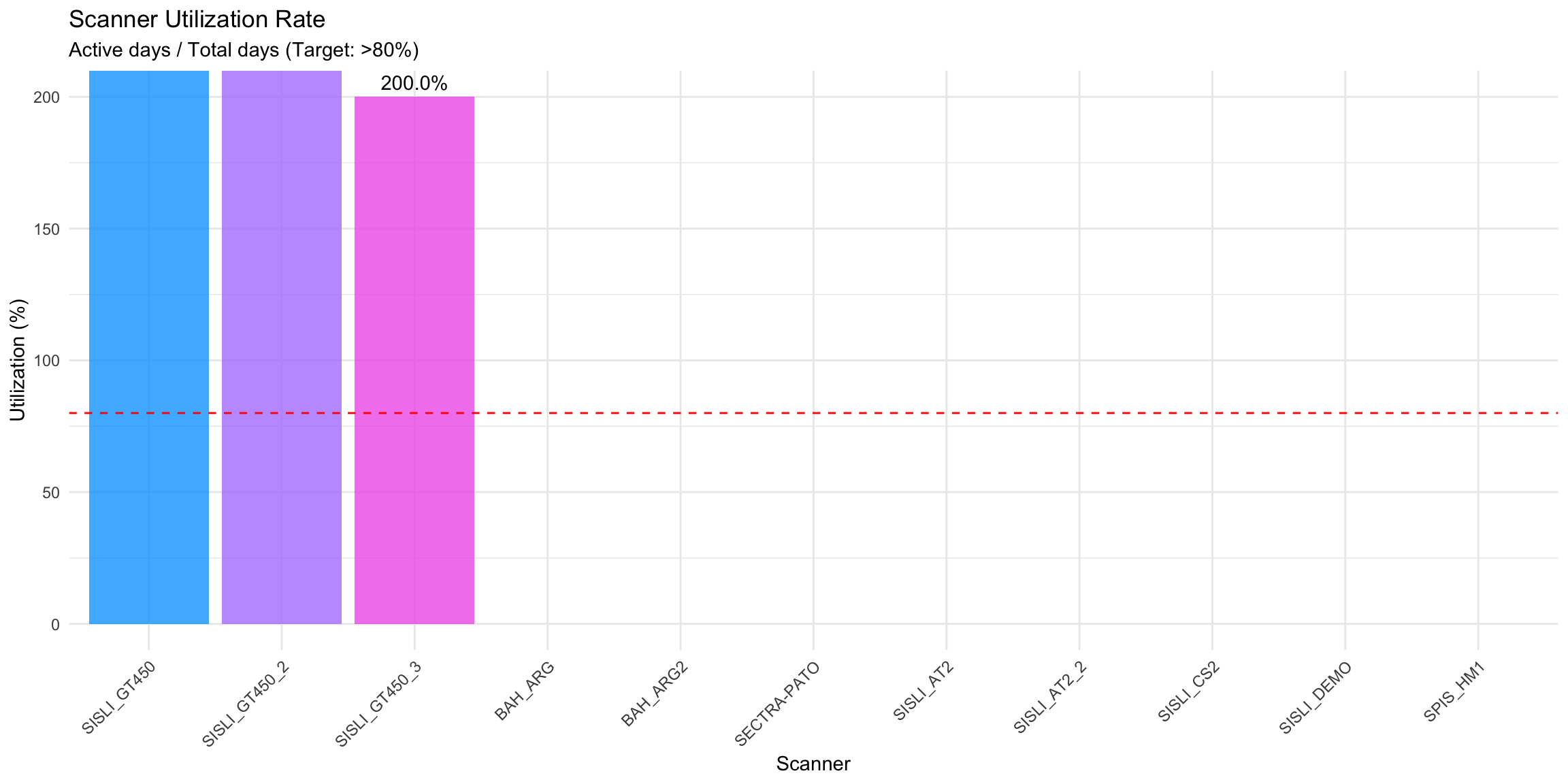
Target: >80% utilization. Low utilization may indicate: - Frequent downtime - Underutilization (need better load balancing) - Recent installation
16.8 Daily Throughput Trends
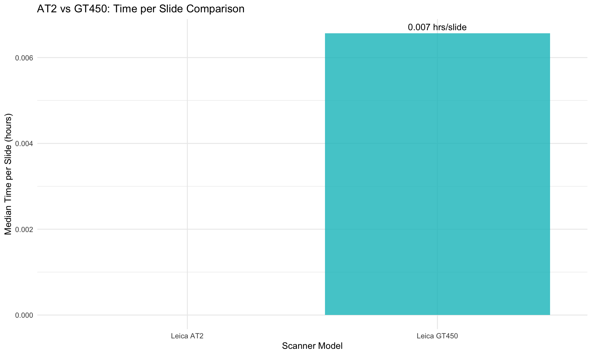
16.9 Model Comparison: AT2 vs GT450
| Model | Cases | Slides | Median Scan (hrs) | Time/Slide (hrs) | IQR | Cases <24h | % <24h |
|---|---|---|---|---|---|---|---|
| Leica AT2 | 352 | 2641 | NA | NA | NA | 199 | 56.534 |
| Leica GT450 | 24452 | 149137 | 0.046 | 0.007 | 0.124 | 22391 | 91.571 |
16.10 Reliability Analysis
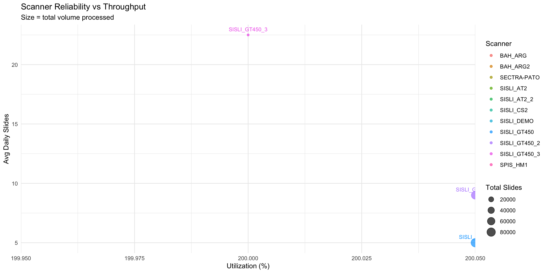
Interpretation: - Top-right quadrant: High utilization + high throughput = best performers - Bottom-right: High utilization but low throughput = potential issues - Top-left: Low utilization but high throughput when active = underused asset
16.11 Load Balance Analysis
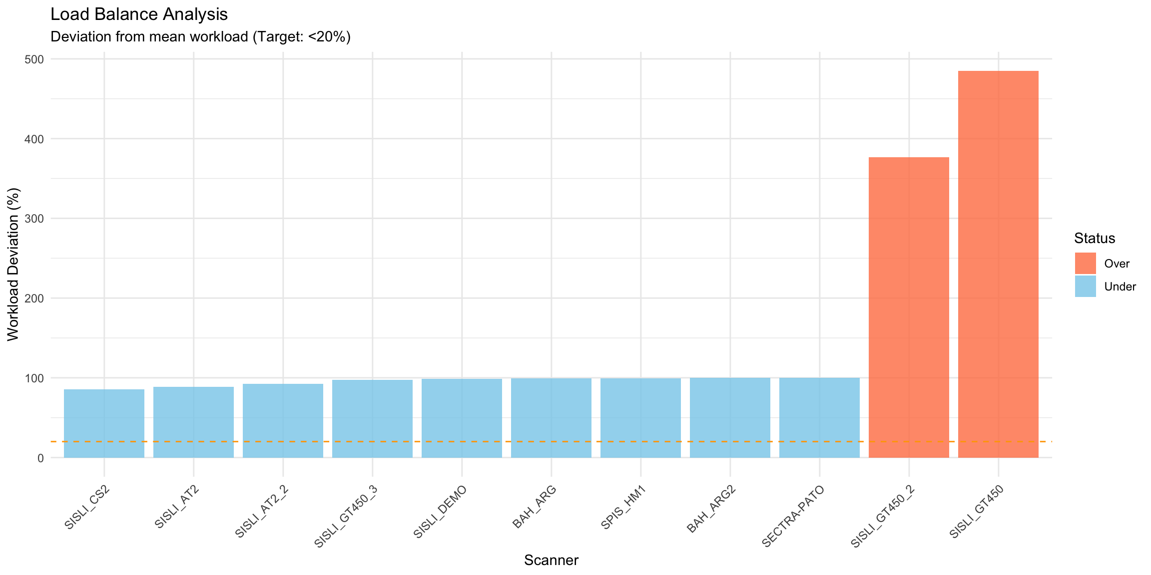
Ideal: All scanners within ±20% of mean workload. Significant deviations indicate: - Underutilized scanners (opportunity for better distribution) - Overutilized scanners (risk of wear and maintenance issues)
16.12 Downtime Analysis
| Scanner | Downtime Events | Total Downtime (hrs) | Avg Per Event (hrs) | Max Downtime (hrs) |
|---|---|---|---|---|
| SS7834 | 143 | 2051.2 | 14.3 | 95.4 |
| SS7833 | 138 | 1953.4 | 14.2 | 95.2 |
| SS45328 | 56 | 962.1 | 17.2 | 50.0 |
| SS45134 | 48 | 850.7 | 17.7 | 41.2 |
16.13 Rescan Rates by Scanner
| Scanner | Total Slides | Rescanned | Rescan Rate (%) |
|---|---|---|---|
| SISLI_DEMO | 19 | 72 | 378.95 |
| SISLI_TECHNOMIND | 8 | 22 | 275.00 |
| SISLI_AT2_3 | 2344 | 3784 | 161.43 |
| SISLI_ARG | 28 | 34 | 121.43 |
| BAH_ARG | 26 | 31 | 119.23 |
| BAH_ARG2 | 70 | 69 | 98.57 |
| SISLI_HMMS | 703 | 597 | 84.92 |
| SISLI_MAG | 353 | 236 | 66.86 |
| SISLI | 776 | 512 | 65.98 |
| SPIS_HM1 | 67 | 32 | 47.76 |
| SISLI_MOTIC | 210 | 90 | 42.86 |
| SISLI_AT2_2 | 78836 | 28697 | 36.40 |
| SISLI_AT2 | 115202 | 29847 | 25.91 |
| SISLI_GT450 | 214337 | 45904 | 21.42 |
| SISLI_GT450_2 | 191522 | 39698 | 20.73 |
| ANTALYA | 234 | 41 | 17.52 |
| SECTRA-PATO | 10216 | 1282 | 12.55 |
| SISLI_GT450_3 | 2542 | 122 | 4.80 |
| SISLI_CS2 | 810 | 17 | 2.10 |
| YSF1 | 1 | 0 | 0.00 |
16.14 Recommendations
16.14.1 For High-Performing Scanners
- Document best practices
- Use as reference for others
- Maximize utilization with priority cases
16.14.2 For Underperforming Scanners
- Schedule maintenance/calibration
- Investigate operator differences
- Consider replacement if chronic issues
16.14.3 Load Balancing Strategies
- Implement automatic load distribution
- Priority routing to most efficient scanners
- Balance to prevent overutilization
16.15 Optimization Strategy
To maximize fleet efficiency:
- Load Balancing:
- GT450: High-volume routine work.
- AT2: Specialized/overflow work.
- QC Efficiency: Automated quality checks on modern scanners (GT450) can potentially reduce QC technician time by up to 94%.
- Predictive Maintenance: Monitor scans-per-error ratio to schedule service before failure.
16.16 Conclusion
Scanner performance analysis reveals opportunities for optimization and investment decisions.