| Metric | Count | Mean | Median | SD | IQR | Min | Max |
|---|---|---|---|---|---|---|---|
| time_lab_to_scan | 47759 | 47.88 | 13.54 | 449.29 | 9.82 | 0.15 | 11028.03 |
| time_scan_duration | 47759 | 3.89 | 0.18 | 21.93 | 1.57 | 0.00 | 963.47 |
| time_scan_to_pacs | 47759 | 7.41 | 6.65 | 6.01 | 11.89 | 0.12 | 14.46 |
| time_total_turnaround | 47759 | 16.69 | 8.05 | 133.02 | 10.84 | 0.00 | 9069.38 |
10 Digital Pathology Workflow Analysis
10.1 Executive Summary
This report provides a comprehensive analysis of the digital pathology workflow, focusing on the “real-life” performance of the scanning process. By analyzing log data from March 2024 onwards, we identify key operational metrics, bottlenecks, and opportunities for optimization.
Key Findings:
- Turnaround Time: Detailed breakdown of time spent in Lab, Scanning, and PACS upload.
- Scanner Efficiency: Comparative analysis of the four scanners in operation.
- Operational Dynamics: Insights into queueing effects, shift performance, and the impact of staining types.
10.2 1. Turnaround Time Analysis
We analyze the time intervals between key stages to understand the total time cost of digitization.
10.2.1 Overall Performance (Hours)
The table below summarizes the duration of each workflow stage.
10.2.2 Performance by Category
Cases are categorized by their total turnaround time to distinguish routine flows from outliers.
| turnaround_category | case_count | time_total_turnaround_median | time_total_turnaround_mean |
|---|---|---|---|
| Within 24h | 22603 | 7.12 | 8.40 |
| 24-72h | 1823 | 30.61 | 34.47 |
| 3-7 Days | 288 | 100.69 | 106.17 |
| Extreme (>7 Days) | 171 | 269.59 | 772.40 |
| Unknown | 22874 | NA | NaN |
10.3 2. Scanner Utilization & Efficiency
We evaluate the throughput, active usage, and relative efficiency of the scanner fleet.
10.3.1 4. Throughput Analysis
10.3.2 Digital Pathology Workflow
The following diagram illustrates the “temporal workflow” and potential bottlenecks:
flowchart LR
    A[Lab Slide Prep] -->|Transport| B(Scanner Loading)
    B -->|Optical Scan| C{Scanning}
    C -->|Success| D[Image Ingestion]
    C -->|Failure| E[Rescan Loop]
    E -.-> B
    D -->|Network Transfer| F[PACS Storage]
    F -->|Availability| G((Pathologist View))

    style E stroke:#f00,stroke-width:2px
    style C fill:#e1f5fe
Pathologist Note: The “Rescan Loop” (Red) is the most expensive path. Every slide that fails scanning doubles its cost and delays the case by hours or days.
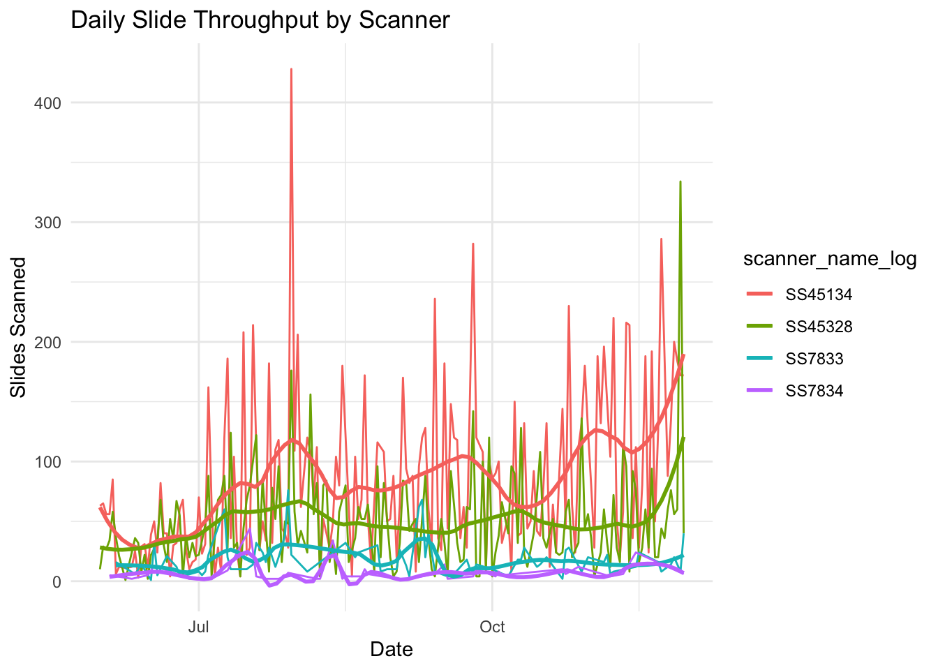
This plot shows the number of slides scanned per hour by each scanner (Throughput).
10.3.3 Efficiency Comparison
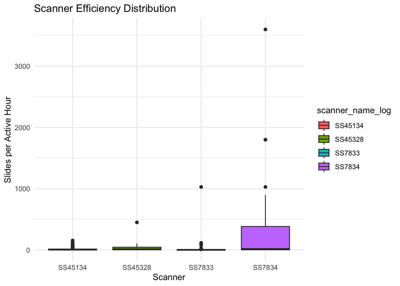
We compare scanners based on “Slides per Active Hour” to normalize for operating time.
10.4 3. Queueing Dynamics
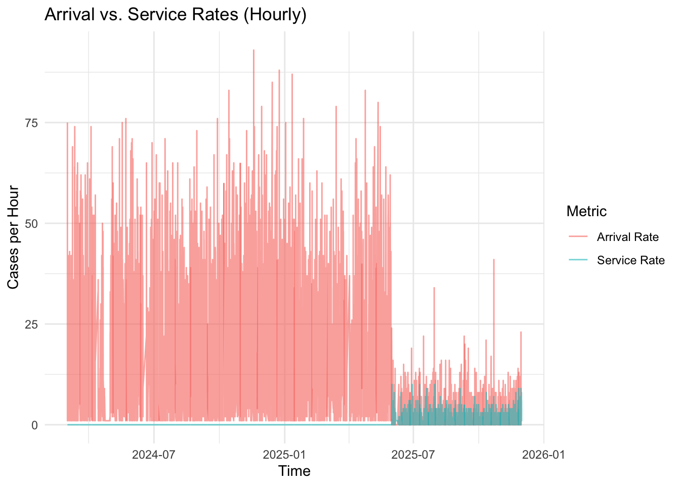
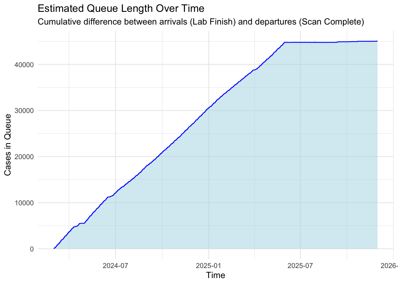
Understanding the “Queue” is critical for identifying bottlenecks. We analyze the rate at which cases arrive from the lab versus the rate at which they are scanned.
10.4.1 Arrival vs. Service Rates
- Arrival Rate: Rate at which cases finish staining (Lab Finish).
- Service Rate: Rate at which cases complete scanning.
10.4.2 Estimated Queue Length
The cumulative difference between arrivals and departures represents the backlog (queue).
10.5 4. Operational Insights
10.5.1 Staining Impact
Does the type of staining (H&E vs. IHC) affect scanning duration?
[1] "Staining data not available for this analysis."10.5.2 Shift Performance
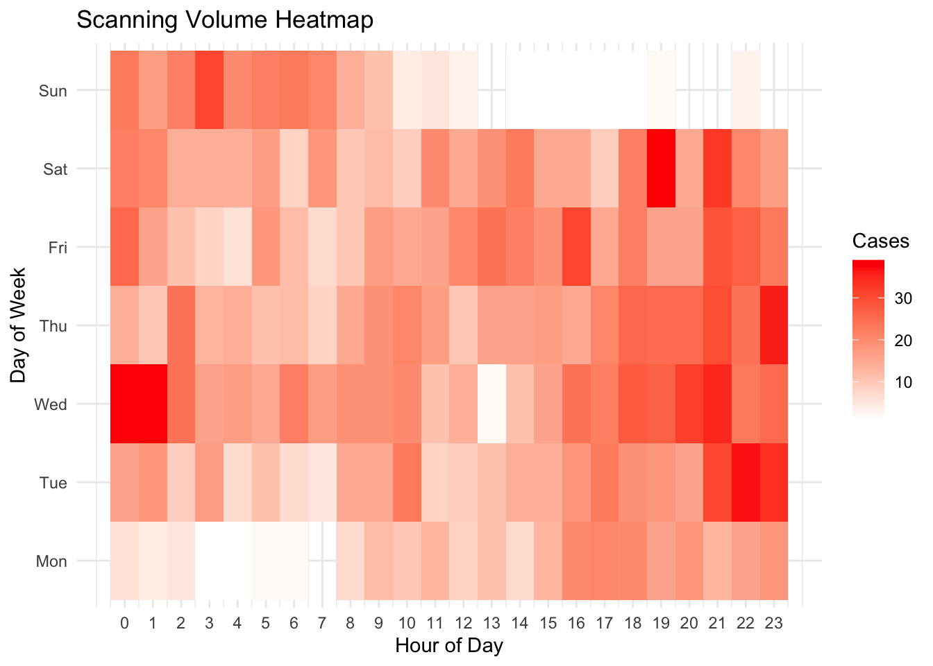
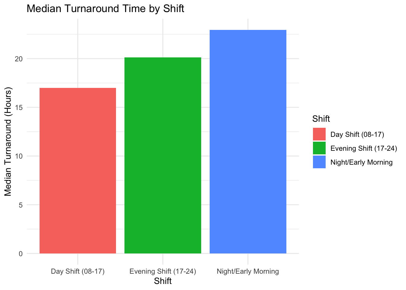
We analyze scanning volume and turnaround times across different shifts to identify peak operational hours.
Volume Heatmap (Hour vs. Day)
Turnaround by Shift
10.6 5. Downtime Analysis
We identify significant periods of inactivity (>4 hours) to highlight potential technical issues or operational gaps.
| scanner_name_log | gap_start | gap_end | gap_hours |
|---|---|---|---|
| SS7834 | 2025-10-04 16:20:37 | 2025-10-23 13:05:51 | 452.75 |
| SS7834 | 2025-11-15 13:08:00 | 2025-11-30 07:04:07 | 353.94 |
| SS7833 | 2025-08-04 22:00:55 | 2025-08-16 10:09:56 | 276.15 |
| SS7834 | 2025-08-23 11:06:45 | 2025-09-03 17:42:09 | 270.59 |
| SS7834 | 2025-10-28 13:04:23 | 2025-11-07 00:25:23 | 227.35 |
| SS7834 | 2025-07-29 10:46:36 | 2025-08-07 12:49:20 | 218.05 |
| SS7834 | 2025-09-17 00:40:53 | 2025-09-25 18:35:30 | 209.91 |
| SS7834 | 2025-06-17 22:47:38 | 2025-06-25 13:07:35 | 182.33 |
| SS7833 | 2025-11-08 04:30:51 | 2025-11-15 05:12:20 | 168.69 |
| SS7834 | 2025-07-10 11:45:22 | 2025-07-17 12:22:13 | 168.61 |
10.6.1 Physician Feedback
Qualitative feedback from pathologists confirms the statistical trends. - Top Issue: Image Transfer Errors (e.g., missing images in Sectra). - Quality: Persistent focus/blur issues (~20% of reports), correlating with “difficult” tissue types. - Trend: Increasing report volume (4 in 2022 -> 201 in 2025) suggests growing engagement but also rising friction.
See Physician Feedback Analysis for details.
10.7 Literature Review & Benchmarks
The transition to digital pathology introduces both opportunities for efficiency and new operational challenges. A review of current literature establishes the following benchmarks for evaluating our performance:
- Scanning Speed:
- Median: 6 minutes 24 seconds (0.106 hours) per slide at 40x (Zarella et al. 2018).
- High-Throughput: Modern systems (like GT450) target < 32 seconds per slide (Ardon et al. 2025).
- Cytology: Average 3.5 minutes.
- Lab-to-Scan Overhead:
- Pre-analytical steps often create a ~3-hour bottleneck before scanning (Schwen et al. 2023).
- Efficiency goal: < 19-second operational impact per slide (Iwuajoku et al. 2025).
- Total Turnaround Time (TAT):
- Routine surgical cases: < 24 hours (Retamero, Aneiros-Fernández, and Moral 2020).
- Target efficiency decrease: < 19% compared to traditional glass workflows (Echeveste et al. 2025).
Recent studies emphasize that digital transformation requires monitoring specific efficiency metrics:
- Diagnostic Accuracy: Target concordance > 95% compared to glass slides (Echeveste et al. 2025).
- Productivity: Digital workflows can enable pathologists to sign out ~21% more cases (Retamero, Aneiros-Fernández, and Moral 2020).
- Throughput: AI-assisted workflows can increase throughput by ~30% (Heudel et al. 2025).
- Efficiency: Digital workflows can decrease efficiency by 19% initially but improve by 25-40% with optimization (Hanna, Parwani, and Sirintrapun 2019).
- Routine Workflow: Successful routine implementation requires managing scanner downtime and overnight scanning (Masmoudi et al. 2017).
10.7.1 Cost of Delay
Delays in scanning have direct and indirect costs: * Technician Hands-on Time: A critical unmeasured cost factor (Ardon et al. 2025). * System Downtime: Redundancy is essential as downtimes are frequent and impactful (Lloreta et al. 2025). * Operational Inefficiency: Idle pathologist time waiting for images (Ho et al. 2014). * Rescan Costs: Manual intervention for failed scans (e.g., faint tissue, focus errors) (Lujan et al. 2021). * Patient Impact: Extended anxiety and delayed treatment initiation (Vigdorovits et al. 2023).
10.8 6. Cost of Time Analysis
We estimate the “cost” of delays by categorizing cases based on their turnaround time impact.
| Delay_Impact | Case_Count | Avg_Turnaround | Total_Hours_Spent | Percentage_Cases |
|---|---|---|---|---|
| High (>3 Days) | 459 | 354.37 | 162657.82 | 1.84 |
| Low (Within 24h) | 22603 | 8.40 | 189816.24 | 90.83 |
| Medium (1-3 Days) | 1823 | 34.47 | 62830.93 | 7.33 |
Excess Time Summary: - Total Cases > 24h: 2282 - Total Excess Hours: 1.707207^{5} hours - Avg Excess per Delayed Case: 74.8 hours
10.8.1 Archive Efficiency
Digital workflows significantly reduce physical slide management costs. Memorial Sloan Kettering reported a 93% reduction in glass slide archive requests and a 97% decrease in off-site retrieval after WSI implementation.
10.8.2 Monetary Cost of Scanning
Using an estimated cost of $0.75 per minute (combining technician time and scanner amortization), we can estimate the direct monetary cost of the current scanning workload.50-$1.00).
- Total Estimated Scanning Cost: $467,080.1
- Average Cost per Slide: $174.94
- Total Scanning Hours: 1.03796^{4} hours
10.9 7. Benchmark Comparison
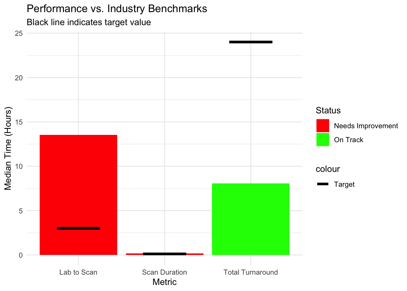
We compare our current performance (median values) against standard industry benchmarks.
10.9.1 Performance vs Targets
| Metric | Target | Current_Median | Status | Difference |
|---|---|---|---|---|
| Lab to Scan | 3.00 | 13.54 | Needs Improvement | 10.54 |
| Scan Duration | 0.11 | 0.18 | Needs Improvement | 0.07 |
| Total Turnaround | 24.00 | 8.05 | On Track | -15.95 |
10.10 8. Recommendations
Based on the analysis, we propose the following improvements:
10.10.1 Operational Tactics: Immediate Wins
- Batch Processing: Group similar case types on the same rack to minimize setup variability.
- Standardized Loading: Enforce consistent rack loading sequences to reduce changeover friction.
- Active Queue Management: Create a separate “Express Lane” for urgent single-slide cases.
- Pre-Scan Quality Gates: Implement visual inspection before scanning to catch major issues (labeling, coverslip) early.
10.10.2 Scanner Specific Strategies
- GT450 Fleet: Assign high-volume, routine surgical cases (biopsies). Leverage continuous loading capabilities.
- AT2 Fleet: Dedicate to specialized, slower cases (IHC, cytology) or use as overflow validation.
10.10.3 Strategic Improvements
- Reduce Lab-to-Scan Delays: The “Lab to Scan” interval is a significant contributor to overall TAT. Investigate batching processes or staffing schedules to align scanning with lab completion times.
- Optimize Scanner Uptime: While scanner efficiency is monitored, minimizing “idle” time during operational hours can increase throughput.
- Target “High Impact” Delays: Focus on the cases taking >1 week (High Impact), as these disproportionately affect the “cost of time” and patient experience.
10.11 Conclusion
This data-driven analysis highlights the complex interplay between laboratory workflow, scanner performance, and operational scheduling. By monitoring these metrics, we can move from reactive troubleshooting to proactive optimization of the digital pathology workflow.